Parameter scans

Luna comes with a flexible interface to run, save and process scans over any parameter or combination of parameters you can think of. A simple example can be found in examples/simple_interface/scan.jl, and we will go through it here. There are only a few necessary steps to run a parameter scan.

First, define the fixed parameters (those which are not being scanned over):

using Luna
import PyPlot: plt

a = 125e-6
flength = 3
gas = :He
λ0 = 800e-9
τfwhm = 10e-15
λlims = (100e-9, 4e-6)
trange = 400e-15

Second, create the arrays which define your parameter scan. A simulation will be run at every possible combination (the Cartesian product) of these arrays. In this example we will do a pressure-energy scan from 50 μJ to 200 μJ in 16 steps and from 0.6 bar to 1.4 bar in steps of 0.4 bar:

energies = collect(range(50e-6, 200e-6; length=16))
pressures = collect(0.6:0.4:1.4)

Third, create a Scan which will store the scan arrays and define how the scan is executed. You must give this a name. In this case, "pressure_energy_example". Scan variables like energies and pressures can be passed at construction time or added later:

scan = Scan("pressure_energy_example"; energy=energies)
addvariable!(scan, :pressure, pressures)

Fourth, run the scan! Here we want to store the output of the scan in a subdirectory of the directory containing the script we're running to avoid clutter. Passing scan and scanidx to prop_capillary will mean that our output files (one for each simulation) are automatically numbered and some information about the scan being run is also stored.

# @__DIR__ gives the directory of the current file
outputdir = joinpath(@__DIR__, "scanoutput")

runscan(scan) do scanidx, energy, pressure
    prop_capillary(a, flength, gas, pressure; λ0, τfwhm, energy,
                   λlims, trange, scan, scanidx, filepath=outputdir)
end

Here, runscan uses the do-block syntax, which wraps its body in a function. In our example this function takes three arguments: scanidx, energy, pressure. Generally, scanidx is always present and uniquely identifies a specific simulation in the scan (it simply runs from 1 to the number of simulations in the scan, length(scan)). The number of subsequent arguments is equal to the number of scan variables you have added to the scan, and their order must match the order in which variables were added to the scan. Alternatively, we could also have wrapped our scan in a function ourselves:

function runone(scanidx, energy, pressure)
   prop_capillary(a, flength, gas, pressure; λ0, τfwhm, energy,
                   λlims, trange, scan, scanidx, filepath=outputdir)
end
runscan(runone, scan)

but the do block syntax is exactly equivalent to this and usually easier.

Running this script will simply run all the simulations, one after the other, in the current Julia session. To alter this behaviour, Scan also takes another argument, the execution mode, which has to be a subtype of Scans.AbstractExec. For example, to run only the first 10 items in the scan, we can use a RangeExec:

scan = Scan("pressure_energy_example", Scans.RangeExec(1:10); energy=energies) # note the second argument here
addvariable!(scan, :pressure, pressures)
outputdir = joinpath(@__DIR__, "scanoutput")

runscan(scan) do scanidx, energy, pressure
    prop_capillary(a, flength, gas, pressure; λ0, τfwhm, energy,
                   λlims, trange, scan, scanidx, filepath=outputdir)
end

Scans can be executed in several ways, which are defined via the various subtypes of Scans.AbstractExec:

• LocalExec: simply run the whole scan on the current machine in a for loop
• RangeExec: run a subsection of the scan as given by a UnitRange (e.g. 1:10 for the first 10 elements)
• BatchExec: divide the scan into batches and run a specific batch (can be used to balance load between processes)
• QueueExec: create a "queue file" which is used to balance load between several processes. This can be executed from multiple processes simultaneously. Alternatively, QueueExec can be made to spawn several subprocesses on the local machine which then use the queueing system to balance load between them.
• CondorExec: create a submission file (aka job file) for an HTCondor batch system running on the current machine and submit it, claiming a specified number of nodes, to execute the scan using a QueueExec.
• SSHExec: use one of the other AbstractExec types but first transfer the file to a remote host via SSH and then execute it. (Note: the remote machine must have Julia and Luna available with the same versions of both, and Julia must be available in a shell via the julia command.) For more details on how to set up execution over SSH, see below.

Command-line arguments

Most of the above execution modes can also be triggered by running the script (the .jl file) from the command line with additional arguments. To show the options, run julia [script] --help where script is your .jl file. As one example, running our scan.jl example in queue-file mode could be accomplished by julia scan.jl --queue, and starting 4 subprocesses to share the queue could be done by julia scan.jl --queue -p 4. Importantly, command-line arguments passed to the script overwrite any explicitly created execution mode within the script.

Manual file naming

The method we used above of passing the scan and scanidx to prop_capillary is the simplest and most reliable way of creating output files in the correct order and with all the necessary information. If you need something else, for example to run a scan including two sequential propagation simulations, you can pass an additional argument filename to prop_capillary. This will then be used instead of the scan name to automatically name the files. In the low-level interface, this is possible via Output.ScanHDF5Output (which is used internally by prop_capillary), which takes a keyword argument fname. Both ways store metadata about the scan in each file (the scan arrays and their order, and the resulting shape of the scan grid).

Processing scan output

After the scan is finished, the individual simulations are stored in separate files. Processing.scanproc streamlines data processing across the scan by automatically combining the results of a single processing function when applied to all files. Continuing with our pressure-energy scan from above, say we want to plot the output spectrum as a function of energy and pressure. To do this, we can run scanproc like this (again using the do-block syntax)

λ, Iλ, zstat, edens, max_peakpower = Processing.scanproc(outputdir) do output
    λ, Iλ = Processing.getIω(output, :λ)
    zstat = Processing.VarLength(output["stats"]["z"])
    edens = Processing.VarLength(output["stats"]["electrondensity"])
    max_peakpower = maximum(output["stats"]["peakpower"])
    Processing.Common(λ), Iλ[:, end], zstat, edens, max_peakpower
end

The function here always takes one argument. This argument is a single read-only HDF5Output which contains the results from one simulation in the scan. The function then processes the results from this one simulation and returns the results. scanproc will combine the output of this processing function for each individual simulation and place it into a grid of the same shape as the original scan. In this example, Iλ has shape (Nλ, Nenergy, Npressure), because the output of the function (Iλ[:, end]) has shape (1484,):

julia> size(Iλ)
(1484, 16, 3)

Because the wavelength axis is the same for all outputs, we don't need to have it repeated. By wrapping it in a Processing.Common, we tell scanproc that it only needs to return one instance:

julia> size(λ)
(1484,)

With this data, we can now plot the energy-pressure scan:

fig, axs = plt.subplots(1, length(pressures))
fig.set_size_inches(8, 2)
for (pidx, pressure) in enumerate(pressures)
    ax = axs[pidx]
    global img = ax.pcolormesh(λ*1e9, energies*1e6, 10*Maths.log10_norm(Iλ[:, :, pidx])')
    img.set_clim(-40, 0)
    ax.set_xlabel("Wavelength (nm)")
    ax.set_ylabel("Energy (μJ)")
    ax.set_title("Pressure: $pressure bar")
    ax.set_xlim(100, 1200)
end
plt.colorbar(img, ax=axs, label="Energy density (dB)")

which will produce this figure: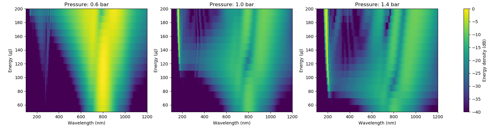

Some outputs from the function may not have the same length for each simulation. For example, the length of propagation statistics arrays depends on how many steps were required in the simulation. To deal with this, we can use Processing.VarLength. Rather than a single multi-dimensional array like Iλ, scanproc will place the results into an array of arrays:

julia> typeof(edens)
Array{Array{Float64,1},2}

julia> size(edens)
(16, 3)

julia> size(edens[1, 1])
(169,)

julia> size(edens[1, 2])
(235,)

For return values which are scalar, like the maximim peak power max_peakpower in our example, the resulting array simply has shape (Nenergy, Npressure):

julia> size(max_peakpower)
(16, 3)

Processing scan results at runtime

Sometimes it is not useful or required to store the whole propagation output for each simulation, but only some result from the simulation is needed. For example, we may only be interested in the output field and not its evolution along the propagation. Especially if we're running very many simulations, storing the evolution and then extracting only the last slice is very inefficient. To make this easy, you can use Output.scansave. This has to be executed within runscan and places arrays and numbers into a grid similarly to scanproc. For instance, to just store the final slice of the frequency-domain field from each simulation, along with the simulation grid, we could have used

runscan(scan) do scanidx, energy, pressure
    output = prop_capillary(a, flength, gas, pressure; λ0, τfwhm, energy,
                            λlims, trange)
    Output.scansave(scan, scanidx; grid=output["grid"],
                                   Εω=output["Eω"][:, end])
end

Note here that scan and scanidx are not given to prop_capillary, so our output lives purely in memory without being saved to disk. If fpath is not explicitly given as a keyword argument to scansave, it automatically names the file. Here it's called pressure_energy_example_collected.h5 and is stored in the current working directory. This file then contains only the grid, the field Eω, and some metadata about the scan:

julia> HDF5.h5open("pressure_energy_example_collected.h5", "r") do fi
         println(keys(fi))
         println(size(fi["Εω"]))
       end
["grid", "scanorder", "scanvariables", "Εω"]
(2049, 16, 3)

Importantly, in our example here this file is less than one megabyte in size, whereas the scanoutput folder totals over 600 megabytes. To store the statistics as well, stats can be given as a special keyword argument to scansave. Because the arrays are not always the same size (see above), in the file these are stored in an array which is large enough to fit the longest and padded with NaNs. The number of actual statisics points available for each simulation is then stored in a special dataset valid_length.

Execution over SSH

Setup steps required:

• On the remote machine, add Julia to your path upon loading even over SSH: add export PATH=/opt/julia-1.5.1/bin:$PATH or similar to your .bashrc file above the usual check for interactive running.
• On Windows, the default version of OpenSSH is v7, but OpenSSH v8 is required to work from within Julia. To install it:
  • Follow these instructions to install the new version.
  • Uninstall OpenSSH via Windows Features. This removes OpenSSH 7 so that Windows finds OpenSSH 8 instead.
• Set up a public/private key pair to enable SSH login without entering a password.